Constrained Portfolio Construction & Factor Attribution

01 / Question and data

What happens after a return estimate?

The project studies the portfolio-construction layer between noisy estimates and feasible portfolio weights: covariance estimation, downside objectives, benchmark-relative risk, turnover, transaction costs, factor exposure, and discrete holding counts.

02 / Walk-forward design

Weights are formed from lagged information

For holding month t, estimates use observations dated through t-1. Missing returns are never replaced with zero. Portfolio weights drift with realized returns before turnover and transaction costs are computed at the next rebalance.

03 / Construction methods

A curated comparison, not a model catalog

04 / Constraints and implementation

Feasibility is part of the research result

The benchmark-relative problem controls position size, ex-ante tracking error, one-way turnover, transaction-cost penalty, and active FF5+momentum exposures. The mixed-integer problem links continuous weights to binary selection variables and checks the selected count and integrality residual.

# src/constrained_portfolio/optimization.py
w = cp.Variable(len(assets))
active = w - benchmark
constraints = [
    cp.sum(w) == 1,
    w >= 0,
    w <= max_weight,
    cp.quad_form(active, cp.psd_wrap(sigma))
        <= tracking_error_limit**2,
]

one_way_turnover = 0.5 * (
    cp.norm1(w - prior) + outside_prior_absolute_weight
)
constraints.append(one_way_turnover <= turnover_limit)
constraints.extend([
    active_factor <= tolerance,
    active_factor >= -tolerance,
])

05 / Public demonstration

The figures show method behavior on synthetic data

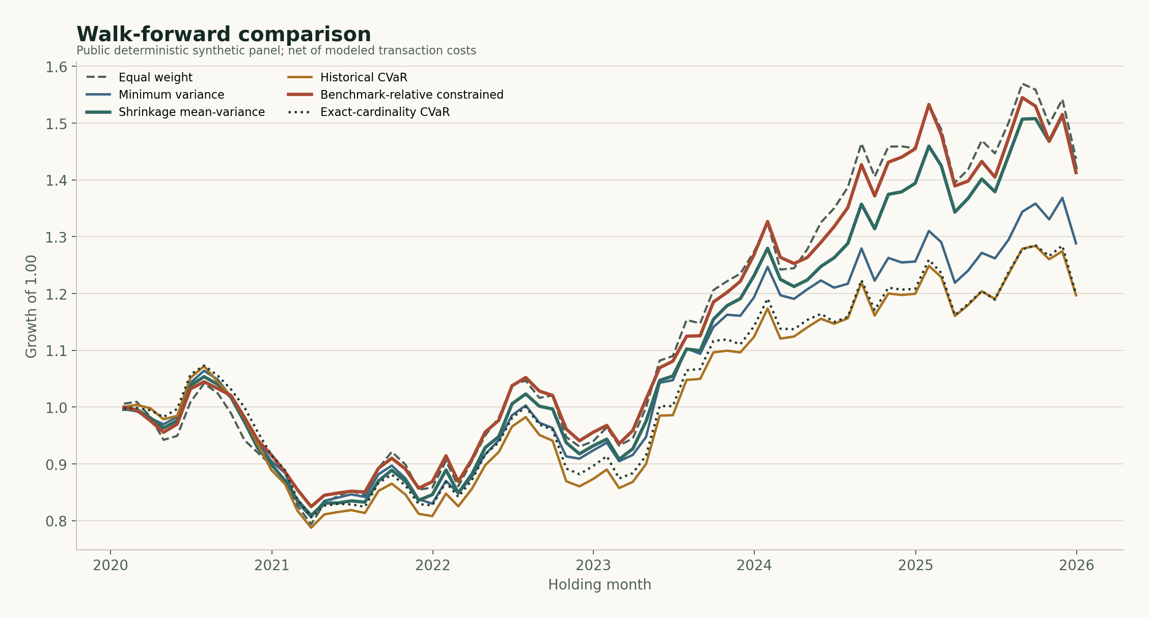
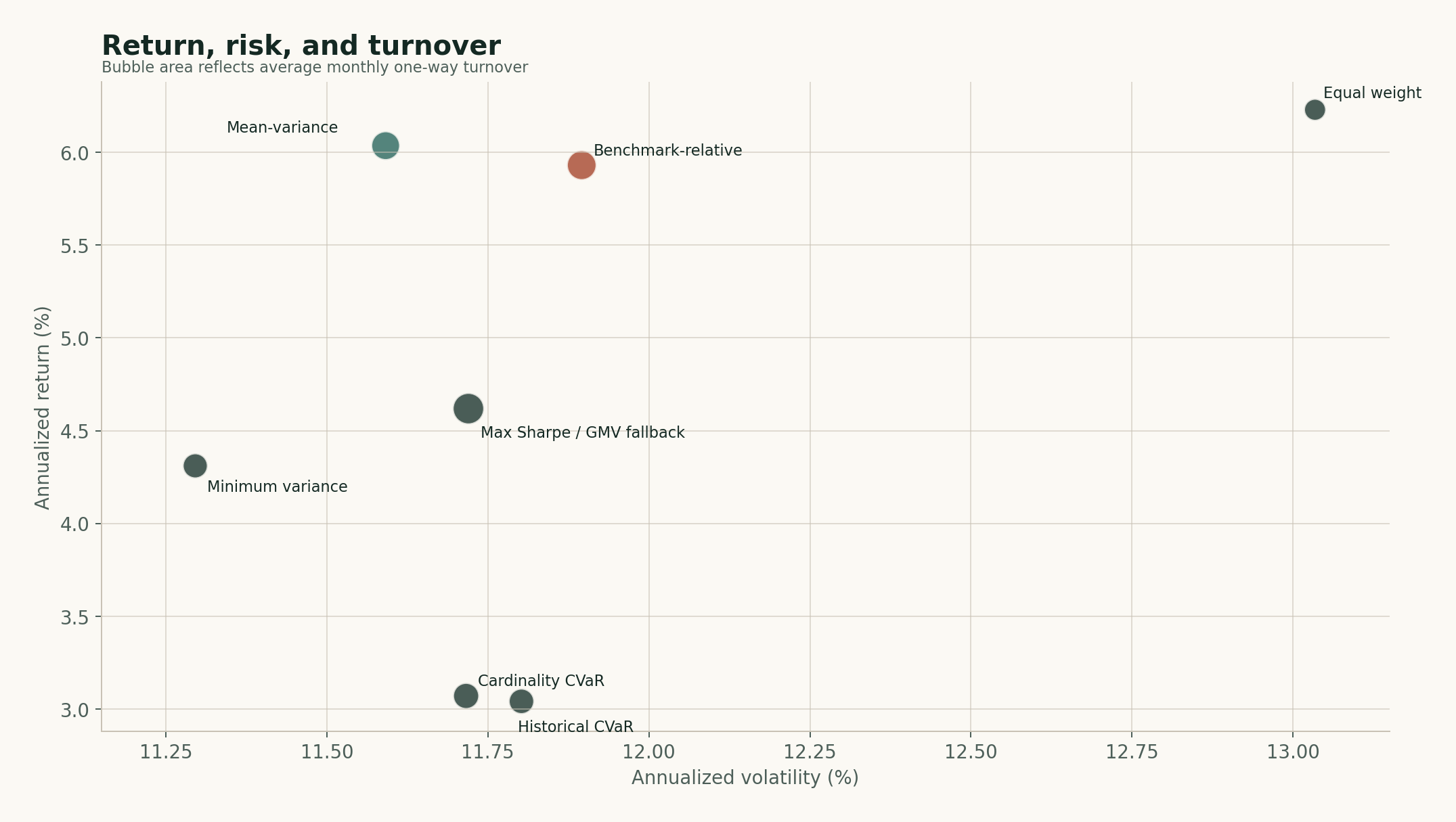
The public run contains 72 monthly decisions from January 2020 through December 2025. Returns include the stated 10 bp one-way turnover cost model. The paths are useful for comparing construction rules, but they are not evidence of alpha or an investable strategy.

06 / Factor attribution

Active-return reconciliation

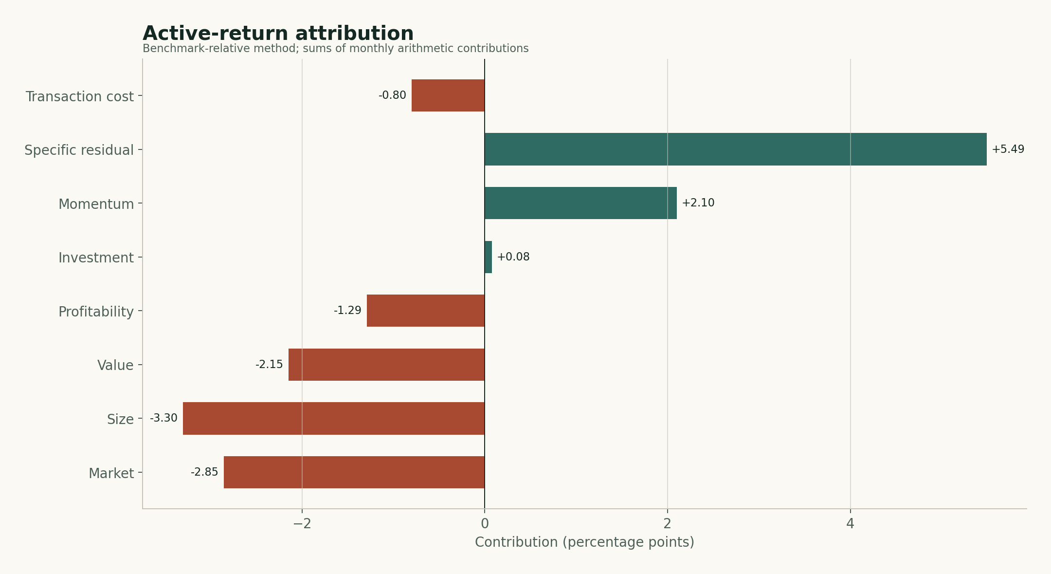
Lagged rolling asset regressions estimate exposures under an FF5-plus-momentum specification; the public demonstration uses synthetic factor series. Monthly active return is decomposed into factor contributions, a specific reconciliation residual, and transaction costs.

07 / Solver checks and uncertainty

Every solution is checked against its stated constraints

The exact-cardinality method selected eight assets in every public-demo month, with maximum integrality residual approximately 3.6e-14 and zero reported MIP gap. Gross return less transaction cost reconciles exactly to net return.

A six-month moving-block bootstrap provides 95% intervals for return, volatility, Sharpe ratio, and maximum drawdown. Every public-demo Sharpe interval crosses zero, so the project does not make a statistical-performance claim.

08 / Limits

Construction mechanics, not an investment claim